Curve interpolation with minimum CV's

[Matt3]

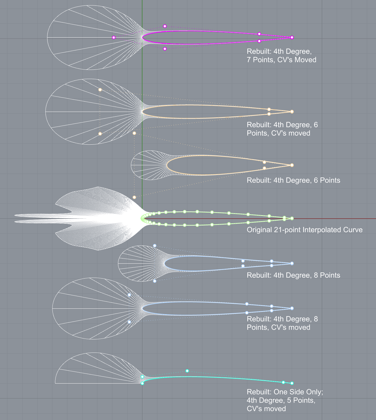
I am trying to model a 4th order 2-D (planar) equation (that also has a square root term) but I want to use only a few (6±) control vertices and preferably with a single span (although maybe I need to consider 2 or 3 spans). 6 points should enable a 5th order curve which should be more than adequate to get an exact match (although the square root term may upend that assessment). In any event, I can calculate (exactly) any CV’s position, tangents, and higher-order derivatives at any and all locations along the curve’s span.

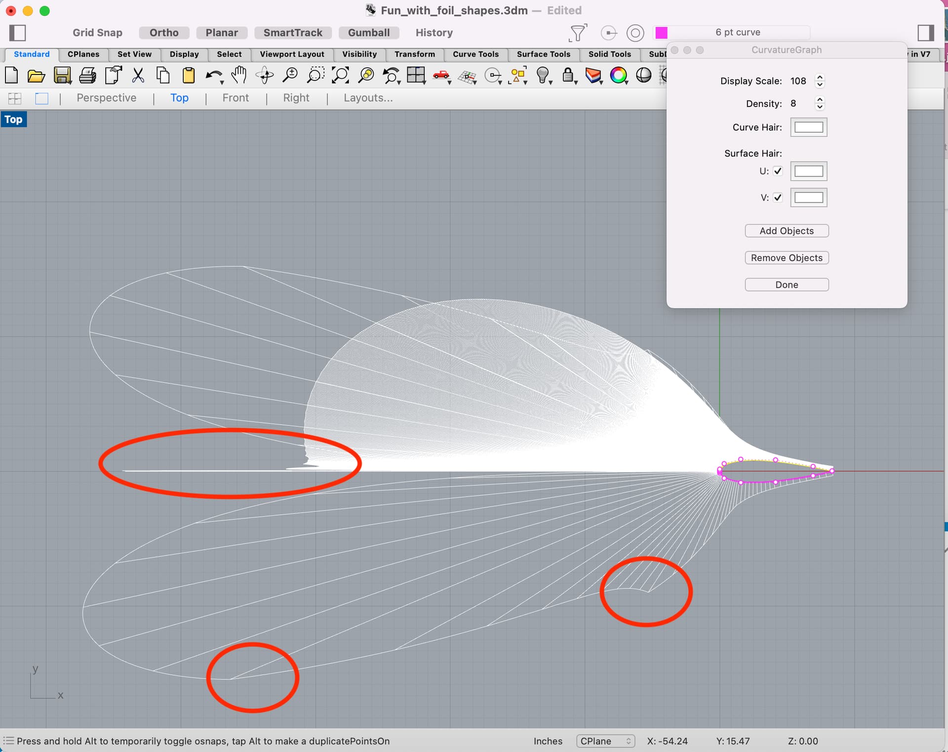
The Grasshopper “tancurve” NURBS interpolation component takes in the position and tangents at each CV, and by adjusting the spacing of the control vertices so they are closer where the curvature is tighter, the curve is still not close to being exact, and the curvature graphs are not as well behaved as I would like to see. The attached screen shot shows different results I am seeing (yellow being the “exact” curve and the green curve getting closest (using the interpolate(t) component). The red one that is closest to yellow uses a mysterious “blend” parameter that can move different parts of the curve around for better localized fit, but setting the “blend” term is still a mystery.

1. So, is there a component that also takes in the higher order derivatives?
2. Is there an alternate/better approach to doing this?

[TomTom (Tom)]

@Matt3

I am trying to model a 4th order 2-D (planar) equation (that also has a square root term) but I want to use only a few (6±) control vertices and preferably with a single span (although maybe I need to consider 2 or 3 spans).

Hi,

could you elaborate what the aim here is?
I think there is a logical error, or I did not understand. A “single-span” NURBS is a Bézier spline. 4th order, Béziers are cubic and have 4 control points. If you increase the order, you increase the amount of control points and of course the exponent of the polynomial.
→ See A Primer on Bézier Curves

§17 of the Primer linked, explains root finding of n-degree Beziers.
You can also modify the weight of a Bezier/Nurbs if rational. This allows you to modify the shape to better fit to a given shape, but also comes with certain drawbacks.

Edit: in a previous version of this post, I mixed degrees with order. The order is of course n+1.

[Matt3]

Objective is to match “exactly” the yellow curve with as few CV’s and spans as possible. If I simply change from 6 points to 5 or 4, the curve match gets even worse at this end (dominated by the square root term), even after adjusting where the points are located. I have not yet explored increasing the number of spans to 2 or 3, which probably will help the curve match, but could make subsequent surface modeling messy.

The more points, the better the match, in general. But, I have not found a way to use the readily available higher order derivatives, which (intuitively) should improve the match with fewer CV’s.

[Matt3]

I probably am using “single span” too crudely, I guess. All I mean by it is that it is a single Rhino curve entity. The “single span” Rhino curve could be higher order than spline or cubic bezier, but still trying to keep the order as low as possible, while remaining “accurate.”

[davidcockey]

Let’s review some terminology and the basics of Bezier and NURBS formulations.

Bezier and NURBS order is always degree +1. Order and degree are positive integers.
Rhino curves are NURBS curves.
Bezier curves and NURBS curves can be of any degree and order.
NURBS curves can have any number of spans.
Degree and order of a NURBS curve are independent of the number of spans.
Any Bezier curve has an exactly equivalent single span NURBS curve.
A Bezier curve of degree n will have n+1 control points.
A NURBS curve of degree n with m spans will have n + m control points.

@Matt3

The “single span” Rhino curve could be higher order than bezier, but still trying to keep the order as low as possible, while remaining “accurate.”

This statement does not make sense in terms of the usual meanings of degree and order.

[Matt3]

@davidcockey

RBS curve.
A Bezier curve of degree n will have n+1 control points.

All that is good. Thank you for the terminology clarification, which I admit to knowing little about.

The core question revolves around how to “accurately” model the given equation in Rhino with the fewest number of control vertices (say 5 or 6) and spans (say 4 or 5), using a parametric/numeric approach, such as with Grasshopper.

[davidcockey]

Interpolating a curve usually means determining a curve which fits exactly through a set of finite number of points.

The higher the degree of the interpolating curve (either NURBS or Bezier) the greater the tendency for oscillations to develop. Degrees greater than 3 are usually not recommended for interpolation. If there are more than 4 points to interpolate through a multi-span NURBS curve of degree 3 or lower is usually recommended.

@Matt3

I have not found a way to use the readily available higher order derivatives, which (intuitively) should improve the match with fewer CV’s.

Your intuition is incorrect. Attempting to use higher order derivatives in interpolation and curve fitting usually leads to oscillations if the process is stable enough to converge to a result.

[davidcockey]

@Matt3

The core question revolves around how to “accurately” model the given equation in Rhino with the fewest number of control vertices (say 5 or 6) and spans (say 4 or 5), using a parametric/numeric approach, such as with Grasshopper.

Method to use in Rhino: (I do not use Grasshopper.)

Generate a set of target points along the target curve. The number of target points should be at least several times the number of control points desired in the fitted curve. More points are generally better as long as the number of points is not very large.

Create a polyline from the target using CurveThroughPts with Degree=1 and Knots=Chord.

FitCrv with Degree=3. Experimentation will be needed to find the Tolerance setting in FitCrv which results in a curve with the desired tradeoff between number of control points and accuracy of the fit. If the resulting curve has a kink where it not desired then increase AngleTolerance in FitCrv, or increase the number of target points and create a new polyline.

[Matt3]

I end up with the same segmented polyline, but with extra control points on each segment. No curve. I must have something set wrong, but I cannot find what it is.

I have something somewhat close using GH, with identifyable issues, but cannot find a way to improve those, except manually.

[TomTom (Tom)]

Curve fitting/approximation is not a really straight-forward topic. A good fitting algorithm also contains a smoothing algorithm to counter the oscillation @davidcockey was explaining.

In practice, manually modelling it is just the faster and more rewarding method. Even in other CAD with better fitting tools, the results are often mediocre.
I often start with an order 3 Bézier at low curved parts, and then increase the degree to better fit, and finally blend the strong curved areas.

Sometimes, e.g. for circles, it is very difficult to fit a non-rational Bézier, simply because of the shape’s nature. To sufficiently match a circle with n.-r. Béziers you would need 4 of them with an order of 7!
This particular examples show that a rational composite spline (e.g. Nurbs) can be superior.

If you still want to automate it, fitting algorithms usually make use of regression methods (Non-Linear Least Squares) or of more abstracted recursive-annealing. For smoothing, I have seen soap-film-dynamics. But in general, this is quite advanced maths. Maybe as someone working with airplane foils you have that knowledge, but my tries in creating own interpolation and approximation algorithms was rather disappointing. In the end, the question remains, does it give you any value for automating it?

Note this topic is 5 years old:

A fast way to approximate a Bezier- or Nurbsspline to an array of points

Hello, It’s one of my first posts here at this forum but I’m frequently hanging out at the grasshopper forum. A while ago I made a plugin, called Advanced Surface Tools for Grasshopper. My intention is to bring some very basic class-A surface functionality to Grasshopper in order to automate some surfacing tasks, which I frequently have to deal with when working with Icem Surf/Rhino -> high quality surface patterns and the ultimate goal: filleting of repetitive structures. One of my main pro…

[Matt3]

The attached picture better describes what I am trying to get the computer to do. The NACA 4-digit airfoil equation I am using is x^4, so I would think 5 points on each side of the mean chord line would be sufficient for a NURBS curve describing one side. I started with a 21-point (on one side) interpolated curve where the 21 points are “exact” locations calculated from the NACA equation, and I cluster more points at the nose where the curvature is greater.

Then, rebuilt curves were generated after both sides were joined. I tried 5, 6, 7, and 8 points on the rebuilt, joined curve. (Note, the joined curve is joined only at the nose, the curve is open at trailing edge - the top half and bottom half do not connect at the trailing edge… a small gap exists there.). The 5-point rebuild did not have the right shape, but the others seemed reasonable. However, initially, the rebuilt curves were very much different in length and width, compared to the target. But, it is relatively quick to manually move the CV’s to get the rebuilt curve to line up on top of the original, calculated curve. So far, the 7-point curve appears to be quickest to manually match the target.

After manually moving the CV’s, the final curves (the top two curves and the 2nd from bottom curve) appear on the screen to be close to the original (middle green one); it seems likely that more fairing by moving the CV’s could get the rebuilt curve to match the target very well. And the rebuilt curve curvature graphs are really nicely shaped compared to the original interpolated curve. I am trying to figure out how to calculate a numerical error value (RMS or similar, maybe an error-moment to help decide which way the CVs move) using Rhinoscript/python.

Even though I used the 2-sided joined curve, it might end up better to work with only one side, as shown by the very bottom curve (4th deg, 5 pts).

Anyway, it seems plausible that, with a Rhinoscript/python or Grasshopper routine, it might be possible to automate the CV movement iterations and numerically check for errors in position, slope, etc. to seed the succeeding iteration. On the other hand, maybe there is a way to directly determine the NURBS curve CV’s and knots directly from the foil parameters themselves.

[davidcockey]

@Matt3

The NACA 4-digit airfoil equation I am using is x^4, so I would think 5 points on each side of the mean chord line would be sufficient for a NURBS curve describing one side.

The NACA thickness distribution equation is a degree four polynomial plus a square root term. The square root term is responsible for the nose shape, and it means that it is impossible to exactly represent the shape by a degree four NURBS curve with control points…