SuperComb: Updates to Curvature Analysis Script for Grasshopper
I’ve made/requested/summoned some updates to my “SuperCombs” script for visualizing curve curvature in Grasshopper. It’s basically an enhanced version of the standard Rhino curvature visualization, giving you more control options and better visual output. Main additions in this update are proportional spacing and fixed minimum and maximum comb line display.
What’s Updated
Better Curvature-Based Density Distribution

Previously, the constant spacing of the comb lines result in sparse in areas with the smallest curvature radius (tight corners), and in blocky display, or required oversampling the entire curve. Now the density of comb lines adjusts based on curvature - tighter curves get more definition with closer spacing, while gentle curves have wider spacing. This helps avoid that “spiky” look around corners that used to force you to increase resolution everywhere.
Dual Spacing Modes with Percentage-Based Approach
I’ve implemented two spacing modes that you can toggle between:
- Constant sampling: Uses a fixed spacing, controlled by the MaxSpacing value
- Proportional sampling: Links the density of comb lines to a percentage of the analyzed curvature radius


The proportional approach uses factors of curvature radius opposed to fixed spacing along the curve. The spacing adjusts proportionally to each curve segment:
MinSpacing(0.005) on a 60mm radius curve gives you 0.3mm spacingMaxSpacing(0.05) on a 215mm radius curve gives you 10.75mm spacing
The toggle lets you switch between these modes depending on your visualization needs.
New CombBias Parameter
There’s a new CombBias parameter (ranges from 0.1-0.9) that controls how the transition between minimum and maximum spacing gets distributed. This helps when you have peaks of maximum curvature that might otherwise dominate the density of the comb line visualization.

Separate BoundaryLineSample Parameter
The boundary line (that extended outer line connecting the ends of comb lines) now has its own sampling parameter. Before, if you used sparse comb sampling, you’d get a blocky, straight-line boundary, in a single segmented single color that just didn’t look great. Now you can have a smooth boundary curve even with sparse comb density. It’s mainly a visual thing, not really affecting the analysis functionality, but makes me feel better to use it. This setting has the biggest effect on performance.
S-Curve Transition
The script now uses an S-curve with adjustable midpoint for transitions between min and max values, which creates more natural-looking transitions between different curvature zones.
Performance
The script runs between 180-200ms to a couple seconds, mostly depending on boundary curve sampling density.
When You Might Use This
This tends to be useful when you need to:
- Get more precise curve analysis than the built-in tools
- Adjust visualization to highlight specific curvature ranges
- Create cleaner curvature visualizations for presentations
A Note on AI-Summoned Development
While I feel the same way about using “AI” in a sentence as “NFT” it seems tired and buzzed out, the functionality and awareness of the Grasshopper environment and writing Python code is quite exceptional. This was not a project that I could have attempted on my own.
This script is over 1,000 lines of well-documented Python code, which was developed with/by Claude by Anthropic. This project required substantial specification work and went through probably 20-30 iterations as ideas were executed and new possibilities discovered. Just a statement of fact, not congratulating myself on hard work, the engine does all the code work to hit the briefed goals.
The process revealed interesting possibilities. For instance, I started with various iterations of cosine-based distribution along curves before discovering that a Hermite ease-out ( learned about this during the course )function worked better for spreading the density of comb lines across the display.
When working with Claude, I found it runs into some limitations around 700 lines of code, which is why the script is now split into discrete, well-labeled sections.
This approach has opened up new possibilities for me in implementing custom Rhino functionality with Grasshopper. The curvature visualization is just one example of what’s possible with this development method.

Annotated radial dimension dots, constant spacing, sparse.
Annotated radial dimension dots, constant spacing, dense.
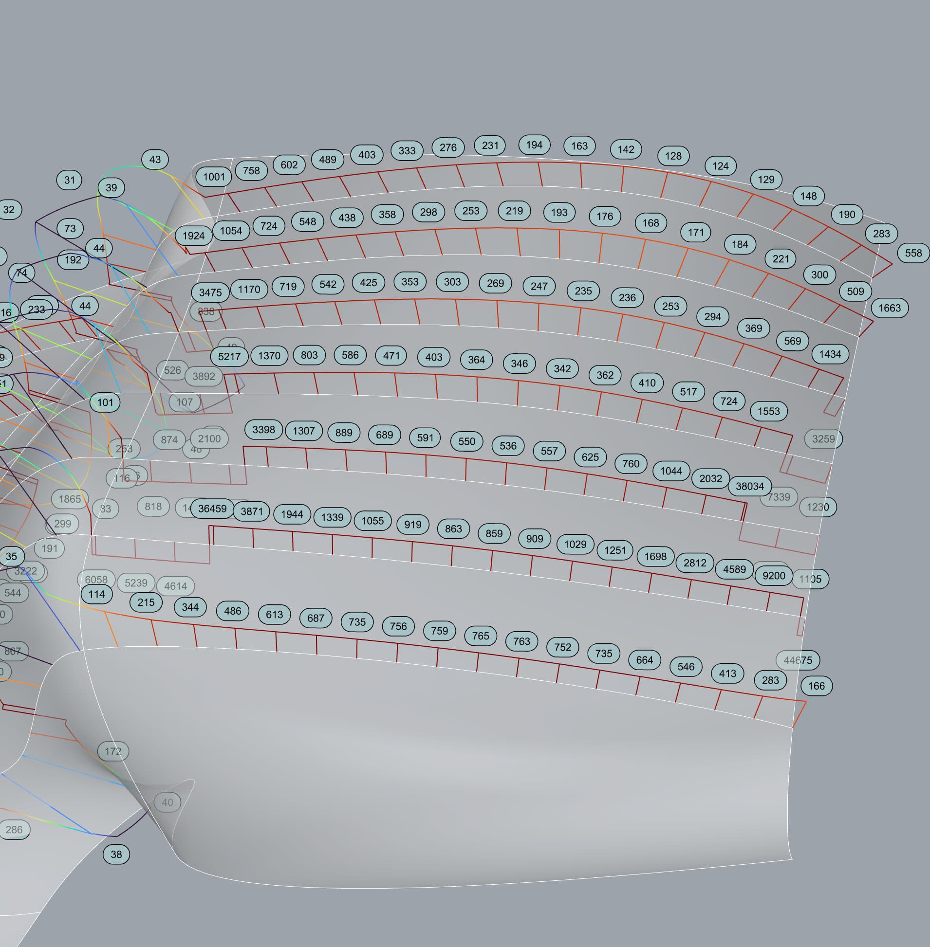
Annotations matching comb line placement, coase resolution in tight radius curvature.

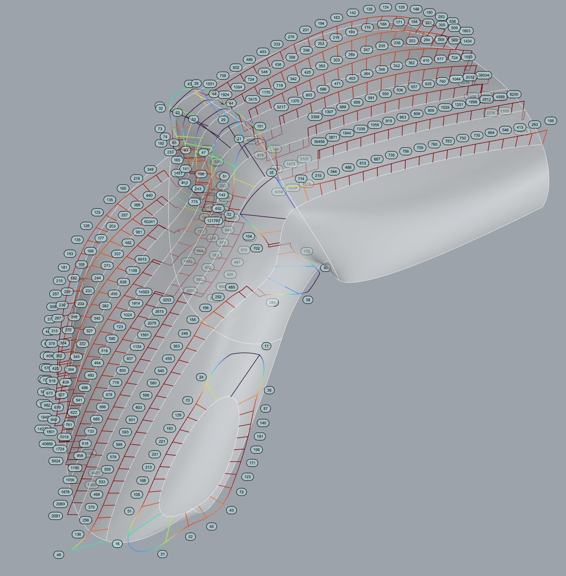
Annotations matching comb line placement, Sparse in larger radius curvature, more dense in smaller radius curvature.
Supercomb.ghx (524.6 KB)