Kangaroo vs. TNA

I´m looking into funicular floor slabs for my master thesis, but first need to clearly understand the aspect of form finding.

Here I am currently experimenting with Kangaroo and RhinoVault 2 and would like to practically understand the differences between these two approaches (virtual force-based physics engine vs. thrust network analysis).
Therefore I created a simple rectangular base mesh with RV2 (with a ~10% sag to the middle in order to avoid invite stresses in the boundary in the resulting funicular shape).

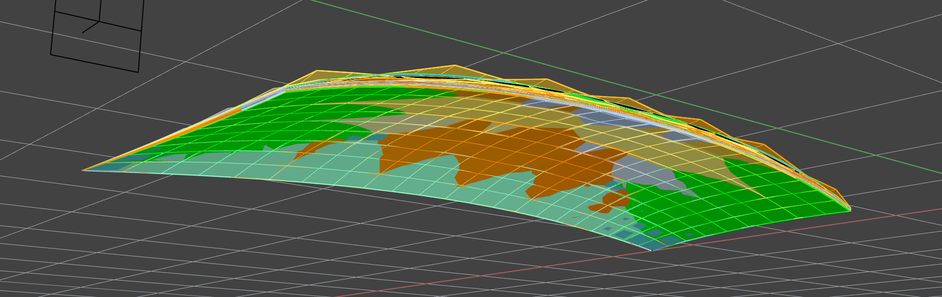
Then I created the “vertical equilibrium” in RV2 and tried to achieve the same shape with Kangaroo (=high stiffness for the edges, a bit longer than the rest length and a small vertical force.) Below you see the RV2 result in purple and the Kangaroo result in green:

Interestingly these two ways of form finding do not result in the same shape, the Kangaroo mesh having less curvature. These are two different approaches to create funicular shapes, so some minor deviations are to be expected.

However I am wondering if I maybe missed sth in the Kangaroo simulation that should be included? AFAIK, the funicular form with a given loading and boundary conditions is exactly calculable? So one of these result must be less optimal?

Any insights would be much appreciated!
Cheers Rudi

rv2_kang.gh (20.8 KB)
rv2_kang.3dm (85.7 KB)

1 Like

The difference becomes more apparent, if a irregular starting mesh is chosen. In this case with the mesh edges follow principal stress directions (a rough approximation for now):

It is visible that the Kangaroo version results more in a cross vault, while the RV2 version results in a dome like vault. Furthermore, the Kangaroo version has its apex not in the middle of the mesh, but in the middle of the side arches.

rv2_kang_2.3dm (60.6 KB)

1 Like

No, there is not a unique optimum here because the problem isn’t defined fully. For a given boundary there are many different perfectly funicular forms possible, depending how the loads are distributed. For example, if you treat the loads as concentrated on the nodes and keep their magnitudes fixed as the shape changes, it is different from having the loads based on the length of edges, and having them update as the lengths change during form finding. With both of these the grid or mesh used will also affect the form.

As long as all the members in the hanging model are in tension, when inverted it gives a compression only form.

For a simple 2d example, take a hanging cable with loads concentrated at 2 points. All these can be purely in tension, just with a different ratio of tension in the middle segment to that in the sides:

3 Likes

Thanks for your response!

Yes, that makes sense. So to be more precise: With a given loading and given load distributions (e.g. uniform load sure to self weight for example)

So your point is, that the reason why those two meshes differ is because of the different load distribution? I read that RV2 is assuming a uniform load as standard… Or is the load distribution in the Kangaroo setup not perfect, due to unequally spaced vertices?

Also another question regarding funicular form finding:
What is the difference between using stiff, but slightly elongated cables vs. cables that can be stretched when loaded? Is the second approach valid?

Also it would super interesting what base mesh was chosen for the form finding of the Mexico airport by F+P. Incredible project… Would have probably been the largest application of form-finding ever.

Thank you! :heart:

1 Like

For the question of

Here the green Length goals are very stiff, but with a total rest length longer than the distance between the anchors, so it forms a hanging curve without the segments stretching.
The red cable has total rest lengths equal to the distance between its anchors, and low stiffness, so the segments stretch.
For both cases the load is kept the same at each vertex.


The green one is the true discretization of a catenary (because the catenary curve is defined as the curve formed by a perfectly flexible inextensible cable hanging under its own weight, with its weight uniformly distributed along its length).
For the red one the segments near the ends are longer because they have stretched more than those nearer the apex, so the weight distribution is no longer uniform by length, since the loads at the nodes have been kept the same.

A third way to do this is to use the DynamicWeight1D instead of the standard Load component.
This lets you use a low stiffness to allow the segments to stretch, but it updates the load at each iteration, so that it is proportional to the changing length. Here this is compared with inextensible segments and equal loads at each vertex, overlaid on a mathematically defined catenary curve for comparison:


Both match the true catenary, just the discretization differs. Now that the solver is stable even for very high stiffness ratios (which were a problem in Kangaroo1) I haven’t often actually found the need to use the DynamicWeight1D goal, but sometimes it can perhaps be convenient to have this option of using zero rest length springs with low stiffness yet still finding true catenaries.

I did write once a DynamicWeight2D triangle, for if you want the loading to depend on the changing area. For form-finding of vaults this would be the difference in form between a gridshell where the weight is distributed uniformly along the linear members (struts/laths) and something like a uniform thickness concrete or masonry shell, where the weight is distributed over the area or panels.
I seem to recall that the actual difference in shape usually ended up being pretty tiny though, and it was only by making the meshing density deliberately very uneven that the difference was visible.

I’d guess that in most practical applications though, live loads likely cause deviations from the pure uniformly distributed load catenary behaviour much larger than these subtleties of discretization, and the material thickness and bending capacity would have to be able to resist these, so the distinction becomes mainly academic.

1 Like

Again thank you for your very detailed answer!

IMO this might be very useful, if one is form finding more complex doubly curved shapes, where the high-stiffness planar starting grid cannot approximate the doubly curved form finding “goal”, due to uneven elongation:

low stiffness:

high stiffness:

So I guess in this case a DynamicWeight2D goal would be very practical? (the low stiffness + low/zero-length constraint would also result in the benefit of actually smoothing out the result)

In the image from my question above, this would be exactly the case. Yes a perfectly regular quad mesh would be solve this probablem. However, on the one side the boundary is not perfectly rectangular due to the supports being cut arc-like and on the other side, the goal is to control specific lines along diagonals / principal stress lines that follow compression forces and thus the mesh itself results in an uneven density, also with some singularities.

Would the DynamicWeight2D goal give a different result for this specific case?

Because if RV2 and Kangaroo are resulting in a roughly equal shape for a perfectly regular quad-mesh, that should also be possible for a non-regular quad mesh I guess? Would be interesting to give DynamicWeight2D a try here. Also tried using the VertexLoads components, but still got the same result…

yes, I was also investigating this fact, here is a non-proportional 2D version with different point loads:

And the same in 3D with asymmetric and point loads assuming 2kN/m² for area and 2kN for point loads for a 5.5m shell:

There are different strategies to handle these non-uniform load cases (adding stiffening ribs, adding creases and thus increasing structural depth… trying to envelop the resulting thrust surfaces) and IMO it should still be the goal to achieve maximally accurate ideal shapes to achieve in lowest possible forces in the structure, especially if in some cases these differences are not negligible.